Advanced Lane Finding

When we drive, we use our eyes to decide where to go. The lines on the road that show us where the lanes are act as our constant reference for where to steer the vehicle. In this project, I develop an algorithm to detect lane lines automatically with a front facing camera. This project is an upgrade to Finding Lane Lines Road.

Programming platform and Libraries: Python and OpenCV.

Methodology

(i) Camera Calibration and Lens Distortion Correction

For camera calibration and lens distortion correction I created a class called Camera

• camera = Camera(directory = 'camera_cal/') initializes the Camera object with the calibration image files
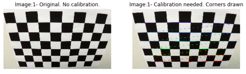
• camera.calibrate() This method uses the loaded images and computes mtx- the camera matrix and dist- the distortion coefficients using cv2.calibrateCamera(). This requires objpoints and imgpoints which are computed using cv2.findChessboardCorners. mtx and dist are made into a dictionary and saved as a pickle object camera_calib.p.
• camera.getCalibration() method loads the calibration file.
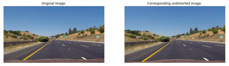
• camera.undistort() is used for correcting the lens distortion in an image.

The images below shows the process of calibration with original and undistorted images.

(ii) Perspective Transform

For obtaining a perspective transform of an image I created the class Transform

• The getPoints() method yields source and destination points for the given image.
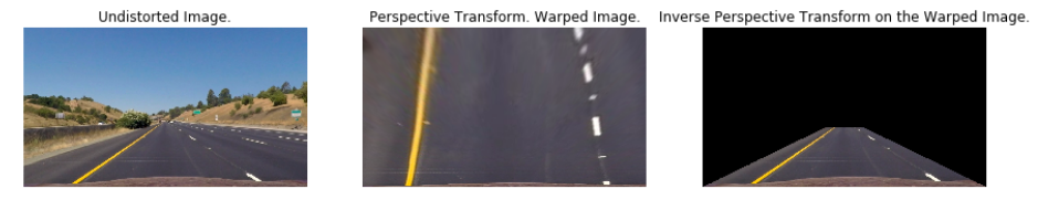
• getPerspectiveTransform() and getInversePerspectiveTransform() yields warped and unwarped images respectively.

The code below outputs source and destination points.

offset = 75
src_pts = np.float32([[w // 2 - offset, h* 0.625], 
                  [w // 2 + offset, h * 0.625], 
                  [offset, h], 
                  [w - offset, h]])

dst_pts = np.float32([[offset, 0], 
                  [w - offset, 0], 
                  [offset, h], 
                  [w - offset, h]])

The figure below shows warped and unwarped images.

(iii) Combined gradient and color thresholds

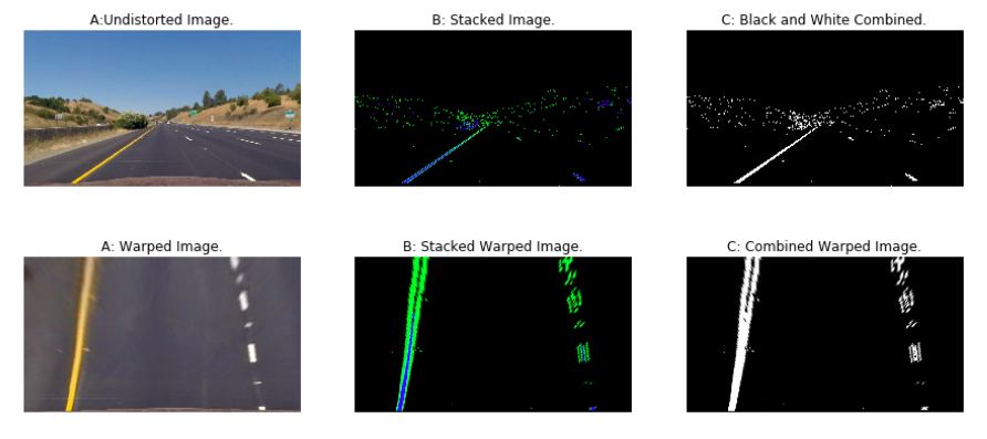
I created the Threshold class for applying combined gradient and color thresholds. The image is converted into HSL space to identify the yellow and white portions since lanes fall into the same color spectrum (Lanes are either white or yellow in color). In addition to the HSL space, Sobel filter in ‘x’ direction is applied to image since the filter in ‘x’ direction detects edges close to horizontal. The figure below shows images with gradient and color thresholds in a combination. The green color in the stacked image represents the gradient threshold region and blue color represents the color threshold.

(iv) Identifying lane line pixel points

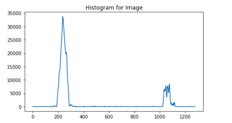
To identify the lane pixels, first we compute the histogram so we know where the lane lines originate and follow them or trace them using sliding windows. I used the sliding window approach to compute the first set of curves and then just used the previous curve parameters to detect new curves. The figure below shows a histogram with two peaks where the lane lines originate.

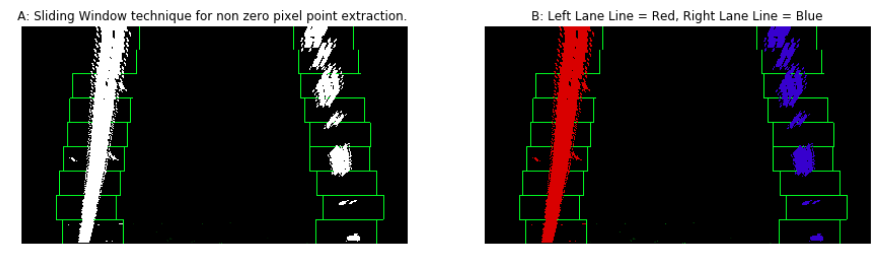
Below is the image showing sliding windows. The sliding windows finds pixel points for lane lines and fits a polygon.

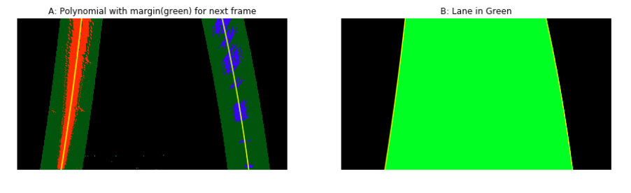
The figure below shows polynomials fit to the pixel points. The lane line in the next frames except for the first one are depicted using the polynomials on the first frame. Also, the lane is sketched out between the left and right lane lines.

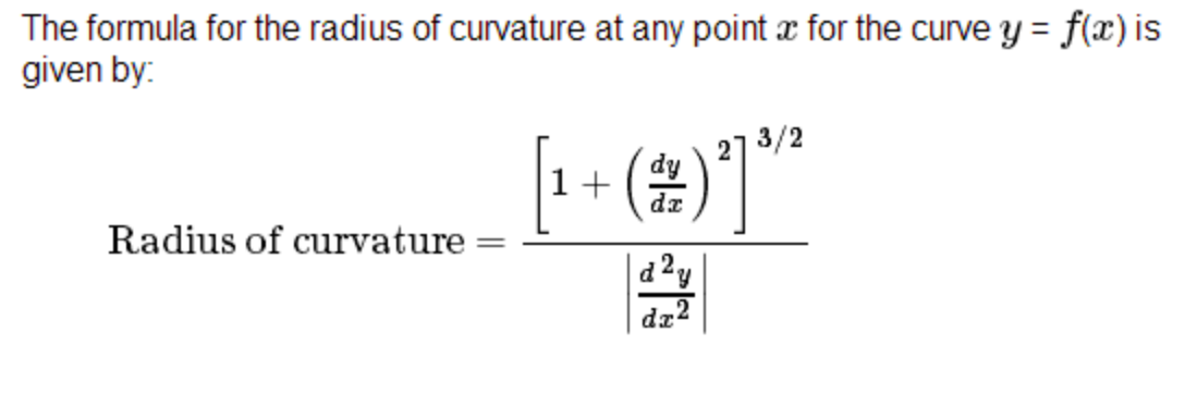
(v) Radius of Curvature

To find the radius of curvature I use the following equations

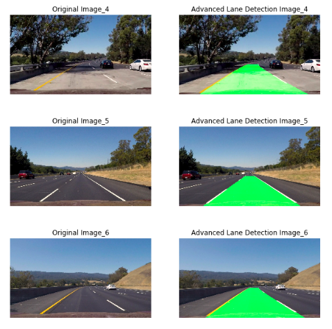
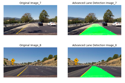
Examples

Conclusion

The method is slow and not robust. Semantic segmentation techniques can be used to identify drivable areas and lane lines.

Code Repository: GitHub