Sim-to-Real SO-101: From 5 Demos to a Working Robot
Most sim-to-real transfer stories start with “we collected thousands of demonstrations.” This one starts with 130 sim seeds and 20 real demos.
The SO-101 is a $300, 5-DOF robot arm with a jaw gripper. The task is pick-and-place: grab a vial off a mat, place it upright in a rack. This is not a research benchmark. It is a real manipulation task that a lab technician would do hundreds of times a day. The question was whether I could build a complete pipeline that goes from a handful of human demos to a working policy on real hardware, using simulation to bridge the data gap.
This post walks through the pipeline I built for the Sim-to-Real SO-101 Workshop, covering where the hard problems actually were and what I had to build to solve them.
The data
Here is the actual dataset breakdown:
| Source | Episodes | Frames | Avg frames/ep | Description |
|---|---|---|---|---|
| Sim seeds (teleop in Isaac Lab) | 130 | ~76,440 | 588 | Teleoperated in simulation via leader arm |
| SkillGen generated | 1,200 | ~319,200 | 266 | Retargeted from seeds to randomized scenes |
| SkillGen filtered | 263 | ~79,163 | 301 | Passed geometric success criteria |
| Real demos (co-training) | 20 | 13,666 | 683 | Physical robot, 3 RealSense cameras |
The co-training dataset (cotrain_v2) combines the rendered SkillGen demos with the 20 real-world demonstrations. The real demos are longer (683 frames vs 301) because physical execution is slower than simulation, and the human operator tends to pause and correct. Both share the same format: 6 joint values + 3 camera views (ego, side, top) at 640x480.
How the three sources compare
The violin plots below show how trajectory characteristics differ across the three data sources.
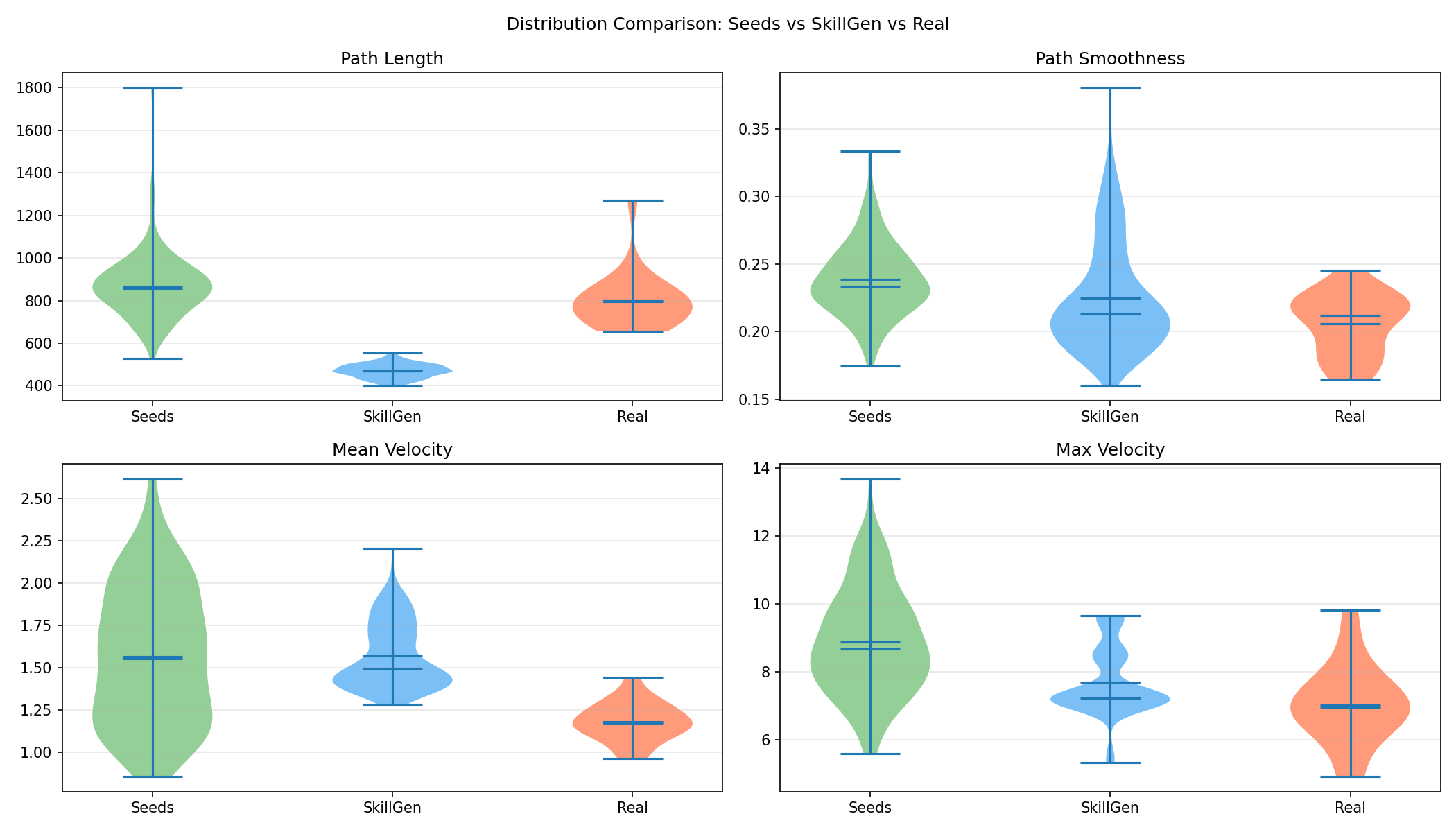
Trajectory metric distributions across the three data sources. SkillGen episodes are shorter and tighter than seeds (path length median ~480 vs ~870) because IK rollout follows the retargeted trajectory without the pauses and corrections of human teleoperation. Real demos have the highest path length variance (650-1250) due to physical execution variability. Path smoothness is similar across all three (0.15-0.35), with SkillGen showing the widest spread. Mean and max velocity are lowest for real demos (median 1.2 and 7.0) because physical servos are slower than simulated joints.
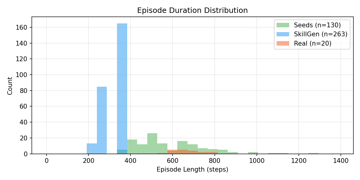
Episode duration distribution. SkillGen episodes cluster tightly around 300-400 steps (n=263), while seed demos spread from 400 to 1000+ steps (n=130). Real demos (n=20) are the longest, peaking around 600 steps. The tight SkillGen distribution is a direct consequence of the IK rollout running at fixed speed without human hesitation.
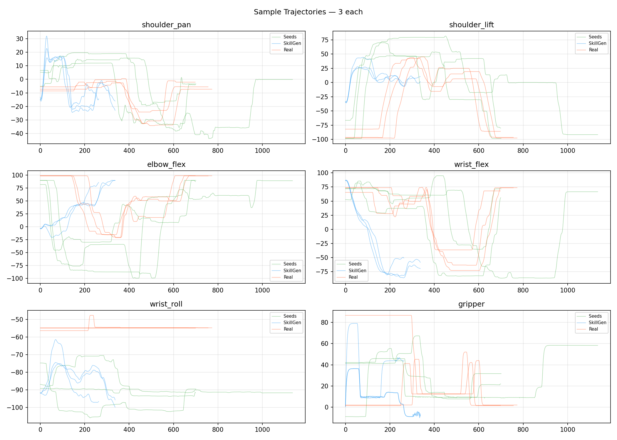
Sample per-joint trajectories (3 episodes from each source). Each subplot shows one joint in motor-degree space. Seeds (green) show the most variation, with wide position ranges and longer durations. SkillGen (blue) trajectories are shorter and smoother, preserving the same joint-space shapes but compressed in time. Real demos (orange) are the longest with plateaus where the operator pauses. The gripper panel (bottom right) is the most telling: seeds and real demos show clear open/close transitions at different timings, while SkillGen gripper commands are sharper because they come directly from the retargeted trajectory without servo lag.
The generation success rate is about 22% (263 filtered from 1,200 generated). That sounds low, but generation_guarantee=true means the pipeline keeps trying until it hits the target count. The 892 failed demos are kept for debugging but excluded from training. Failures are mostly IK tracking divergence on extreme object poses or dropped vials during place.
The pipeline at a glance
Each stage reads its parameters from YAML config, with no hardcoded constants anywhere. The pipeline is orchestrated by Prefect and every stage is resumable: if rendering crashes at demo 147, it picks up at 148.
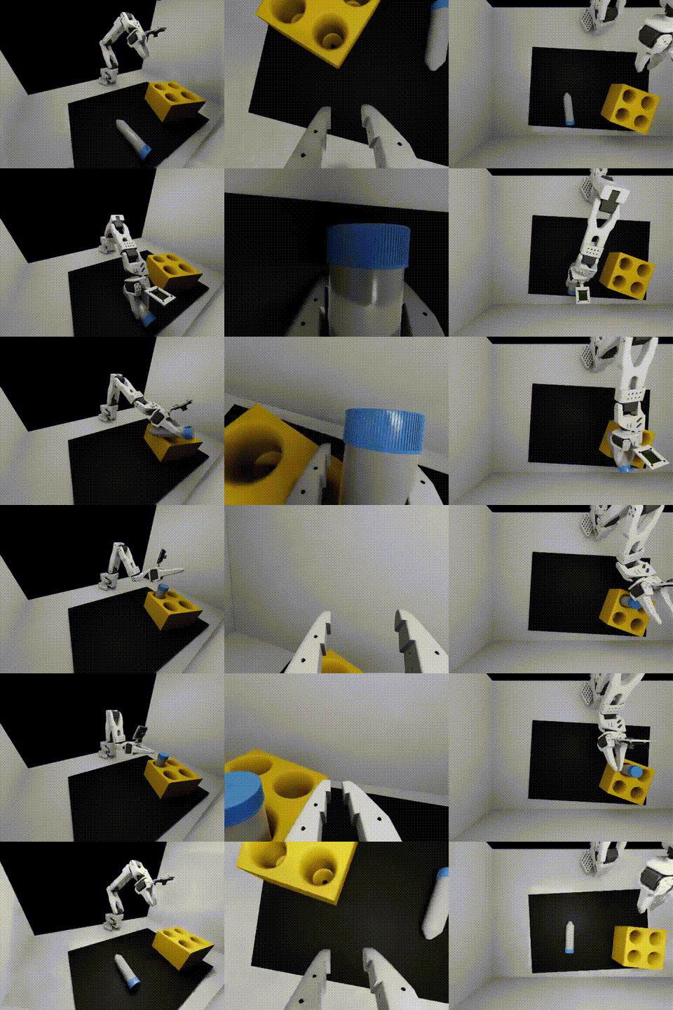
SkillGen-generated episode rendered in Isaac Sim (side, ego, top cameras).
Collecting seeds: 5 minutes of teleoperation
The SO-101 has a leader-follower setup. You physically move a leader arm and the follower mirrors it via Feetech servos over serial at 30 Hz. I record 3-5 demonstrations of the pick-and-place task, storing joint positions as HDF5 files.
Five demos is not a typo. The whole point of the pipeline is that you do not need hundreds of human demonstrations. You need a few good ones that capture the skill structure, and simulation handles the rest.
How SkillGen works
SkillGen is the demo multiplier. It turns 5 human demonstrations into 200+. The idea comes from Mandlekar et al. (2023), adapted here for Isaac Lab and the SO-101’s kinematic constraints. Understanding how it works requires being precise about what a demonstration actually contains.
A human demonstration encodes two things: (1) the skill structure, meaning the approach angle, grasp timing, wrist orientation at contact, and place trajectory; and (2) the spatial binding, meaning where the objects happened to be during that specific demo. SkillGen separates these. It keeps the skill structure and rebinds it to new object configurations.
The three-stage pipeline
Stage 1: Forward kinematics replay. Take a seed demonstration’s recorded joint angles and drive them through the Isaac Lab simulator. At each timestep, a FrameTransformer reads the end-effector pose in the robot’s base frame. The output is the original EE trajectory as a sequence of SE(3) poses, capturing positions and orientations in 3D space.
This happens in skillgen/fk_replay.py. The simulator is not stepping physics here; it is just computing forward kinematics to recover what the end-effector was doing during the original demonstration.
Stage 2: SE(3) retargeting. This is the core math. Given the seed’s object pose \(T_{\text{seed}}\) and a new randomized object pose \(T_{\text{new}}\), compute the rigid displacement:
\[\Delta T = T_{\text{new}} \cdot T_{\text{seed}}^{-1}\]Then apply \(\Delta T\) to every pose in the EE trajectory. The rotation component uses Shepperd’s method for numerically stable quaternion extraction from the rotation matrix. This matters because naive extraction degrades near singularities (0 and 180 degree rotations), and I apply this transform hundreds of times per trajectory.
What this preserves: the approach vector relative to the object, the grasp orientation, the lift height, the place motion shape. What changes: where in the workspace these motions happen. The skill transfers; the coordinates do not.
This happens in skillgen/retarget.py. It is pure math with no simulator dependency, a torch-only module that operates on batched pose tensors.
Stage 3: IK rollout. The retargeted EE trajectory is now in Cartesian space, but the robot needs joint-space commands. An IK controller tracks the trajectory, computing joint angles at each timestep that achieve the desired EE pose. This is where the 5-DOF constraint makes things hard (more on this below).
This happens in skillgen/ik_rollout.py, running inside the Isaac Lab environment with physics enabled. The IK controller commands the robot, physics steps forward, and the resulting joint positions become the new demonstration’s action sequence.
Subtask decomposition and source selection
A single pick-and-place has two subtasks: grasp and place. For multi-vial tasks, that is 2 subtasks per vial. SkillGen decomposes each seed demo into these subtasks and selects sources per-subtask, not per-episode.
The selection uses k-nearest-neighbor matching (k=3) on the object pose relevant to each subtask. So for a generated episode where vial 1 is at position A and the rack is at position B, the grasp subtask might draw from seed demo 2 (whose vial was closest to A) while the place subtask draws from seed demo 4 (whose rack was closest to B).
This is what gives SkillGen combinatorial coverage. Five seeds with 2 subtasks each produce up to \(5 \times 5 = 25\) unique subtask combinations per object configuration. Multiply that by domain randomization over object poses, and 200 diverse demonstrations are straightforward to generate.
Generation runs with generation_guarantee=true and num_trials=20. It keeps retrying until the target demo count is reached, discarding failed attempts where IK tracking diverged or the vial was dropped.
The 5-DOF IK problem
The SO-101 has 5 arm joints controlling a 6-DOF end-effector pose. One degree of freedom, rotation about the gripper’s approach axis, is kinematically uncontrollable. Standard IK solvers either fail or produce degenerate solutions that spin the wrist unnecessarily.
I built a swappable IK backend system (strategy pattern, factory-driven by ik.yaml) with two implementations:
Jacobian backend (default) uses the full 6x5 PhysX Jacobian with damped least-squares. The solver computes:
\[\Delta q = J^T (J J^T + \lambda^2 I)^{-1} \cdot W \cdot e\]where \(J\) is the 6x5 Jacobian, \(\lambda = 0.05\) is the damping factor, \(W\) is the task-space weight matrix, and \(e\) is the 6D pose error (position + orientation). The weights are [1, 1, 1, 0.5, 0.5, 0.2], giving full position priority with partial rotation. Each joint update is clamped to max_delta_q = 0.1 rad to prevent large jumps.
The Jacobian itself comes from Isaac Lab’s PhysX integration. One important detail: the Jacobian’s row layout is [0:3] = translation, [3:6] = rotation. This is not documented clearly, and I initially had them flipped, which produced subtle tracking errors that only showed up during fast motions.
cuRobo backend (GPU-accelerated) uses NVIDIA’s cuRobo library to provide a GPU-parallel IK solver. It runs 32 seed configurations through 100 gradient iterations simultaneously, using PoseCostMetric(reach_partial_pose=True) to accept solutions where the uncontrollable rotation axis does not match. The weight vector [1.0, 1.0, 1.0, 0.05, 0.05, 0.05] follows cuRobo’s convention of rotation-first ordering [rot_x, rot_y, rot_z, pos_x, pos_y, pos_z], which is the opposite of the Jacobian backend’s position-first ordering. Getting this wrong produces IK solutions that prioritize orientation over position, resulting in trajectories where the arm reaches the right wrist angle but misses the vial by centimeters.
The backend swap is config-driven: change backend: jacobian to backend: curobo in ik.yaml and the factory function handles the rest. Both backends implement the same solve(robot, env_id, curr_pose, target_pose) interface and return joint positions.
Adaptive rotation scaling
One fix that had an outsized impact on success rate: during the place phase, when the arm is descending toward the rack, large position errors caused the rotation objective to dominate the Jacobian pseudoinverse. The arm would spiral instead of descend, trying to nail the wrist angle while drifting off-target in XYZ.
The fix is continuous, not a hard switch. When position error exceeds 1cm, rotation weight scales down by max(0.01 / position_error, 0.05). At 20cm of position error (start of a place motion), rotation weight drops to 5% of nominal. At 1cm (final alignment), it is back to 100%. Position gets priority for large motions; orientation tracking kicks in for fine positioning.
This alone took success rate from roughly 40% to 90% on generated demonstrations.
How cuRobo works (and where it fits)
cuRobo is NVIDIA’s CUDA-accelerated robot motion generation library. It solves two problems that matter for this pipeline: inverse kinematics and collision-free motion planning. Both run entirely on the GPU, which makes them fast enough to use inside a simulation loop.
cuRobo’s IK solver
Classical IK solvers (Jacobian pseudoinverse, damped least-squares) are iterative. They take one step at a time toward the target pose. cuRobo’s approach is different: it treats IK as a nonlinear optimization problem and solves it with L-BFGS (a quasi-Newton method) on the GPU.
The solver starts from multiple seed configurations (I use 32) and optimizes them in parallel. The cost function is a weighted sum of:
- Position cost: L2 distance between current and target EE position
- Orientation cost: geodesic distance between current and target rotation (using quaternion difference)
- Self-collision cost: penalty for collision sphere overlaps along the kinematic chain
- Joint limit cost: penalty for approaching joint limits
For the SO-101’s 5-DOF arm, the reach_partial_pose flag tells the solver to relax the orientation cost along the uncontrollable axis. Without this, the solver wastes optimization iterations trying to achieve an orientation that the robot physically cannot reach.
The solver returns the best solution across all 32 seeds after 100 gradient iterations. This takes about 2ms on an RTX 5090, compared to 0.5ms for the Jacobian backend. It is slower per-call, but the solutions are higher quality because they account for self-collision and joint limits, which the Jacobian solver ignores.
cuRobo’s motion planner
The motion planner generates collision-free trajectories between waypoints, which SkillGen uses for transitions between subtask phases (for example, moving from the post-grasp lift to the pre-place position above the rack).
The planner works by optimizing a trajectory (sequence of joint configurations) with the same L-BFGS optimizer, but with additional costs:
- Swept-volume collision: checks the entire trajectory for collisions with the environment, not just individual configurations
- Smoothness: penalizes large joint velocity and acceleration
- Time optimality: controlled by
time_dilation_factor(I use 0.5 for slower, smoother transitions)
The robot is represented as a set of collision spheres attached to each link (defined in so101_curobo.yml). The environment (table, rack, vials) is represented as primitive shapes synced from Isaac Lab at each planning call.
Frame transform gotcha
cuRobo plans in the robot’s URDF base frame. Isaac Lab reports all poses in the world frame. In multi-environment setups (running N parallel simulations for faster data generation), each environment has a different world-frame origin.
This mismatch has to be handled in three separate code paths:
- plan_motion: target poses must be transformed from world frame to base frame before planning
- get_planned_poses: planned poses must be transformed back to world frame for Isaac Lab
- _sync_object_poses: obstacle positions must be transformed to base frame for collision checking
I maintain a per-environment frame cache that stores the world-to-base transform for each parallel env. Getting any one of these three transforms wrong produces plans that look correct in single-env testing but diverge with multiple envs. This is a bug that is easy to miss if you only test with num_envs=1.
cuRobo on Blackwell (RTX 5090)
cuRobo’s L-BFGS optimizer uses a fused CUDA kernel that internally assumes v_dim >= 7 (the number of joint dimensions). This holds for standard 6-7 DOF arms but crashes on the SO-101’s 5 DOF with a dimension mismatch inside the kernel.
The fix: monkey-patch LBFGSOpt.__init__ to set use_cuda_kernel = False, falling back to a pure PyTorch implementation. This also requires disabling CUDA graphs (use_cuda_graph=false) since they are incompatible with the PyTorch L-BFGS fallback on sm_120. The patch lives in so101_curobo_planner_cfg.py and is applied at config load time, isolated from the rest of the pipeline.
Smoothing, filtering, rendering
After generation, the raw trajectories need processing before they are useful as training data.
Smoothing uses a Savitzky-Golay filter with window=21, order=3, applied to arm joints only. The gripper joint (index 5) is explicitly excluded because smoothing destroys the sharp open/close transitions that the gripper needs. A “smoothly closing” gripper cannot generate enough grip force to hold a 20-gram vial. This was a non-obvious failure mode. The trajectories looked better after smoothing, but the policy trained on them could not grasp.
Filtering runs geometric validation to check that the vial actually ended up in the rack: horizontal distance less than 7cm from rack center, vertical offset between -2cm and +10cm above the rack surface, and an upright check (vial’s up-axis z-component > 0.5). Simple thresholds, but they catch the failure modes that matter.
Rendering replays the filtered trajectories through Isaac Sim with three cameras (ego/wrist, side, top) capturing 640x480 RGB frames. Joint states are written directly to the articulation (bypassing the PD controller) for deterministic replay. This is 10-30x faster than stepping physics because it only needs sim.render(), not sim.step().
One physics detail that took real debugging time: PhysX’s default contactOffset of 2cm creates an invisible collision envelope around objects. The gripper’s envelope would overlap with the rack’s envelope at distance, pushing the rack away before any visible contact. This “phantom push” only showed up in certain approach angles. Setting rack contact_offset to 0.00001m fixed it, but finding it required visualizing PhysX’s narrow-phase collision geometry, which is not rendered by default.
Training: GR00T N1.6-3B fine-tuning
The generated demonstrations get converted to LeRobot v2.1 format and fed into NVIDIA’s GR00T N1.6-3B vision-language-action model. The architecture: an Eagle vision encoder processes the three camera views, a 2B-parameter LLM fuses vision tokens with the language instruction (“Pick up the vial and place it in the rack”), and a 1.1B-parameter diffusion transformer head predicts action chunks in joint space.
I freeze the LLM and vision encoder entirely. They already understand visual scenes and language from pre-training. Only the projector and diffusion head get fine-tuned. This means roughly 280 demonstrations (263 sim + 20 real) are enough to teach the model a new manipulation skill without degrading its general capabilities.
| Parameter | Value | Why |
|---|---|---|
| Optimizer | paged_adamw_8bit | Fits in 32GB VRAM with gradient checkpointing |
| Batch size | 32 (x2 grad accum) | Effective batch of 64 for stable DiT training |
| Learning rate | 1e-4, cosine decay | 5% warmup, decays to near-zero at 20K steps |
| Training steps | 20,000 | 2.4 hours on a single RTX 5090 |
| Input | 3 cameras + 6-DOF state + language | Ego, side, top views; 5 arm + 1 gripper |
| Output | Action chunk (T=16) | Multi-step prediction for temporal consistency |
Training metrics
The training script reads all hyperparameters from training.yaml. MLflow tracks loss, gradient norm, learning rate, and system metrics throughout training.
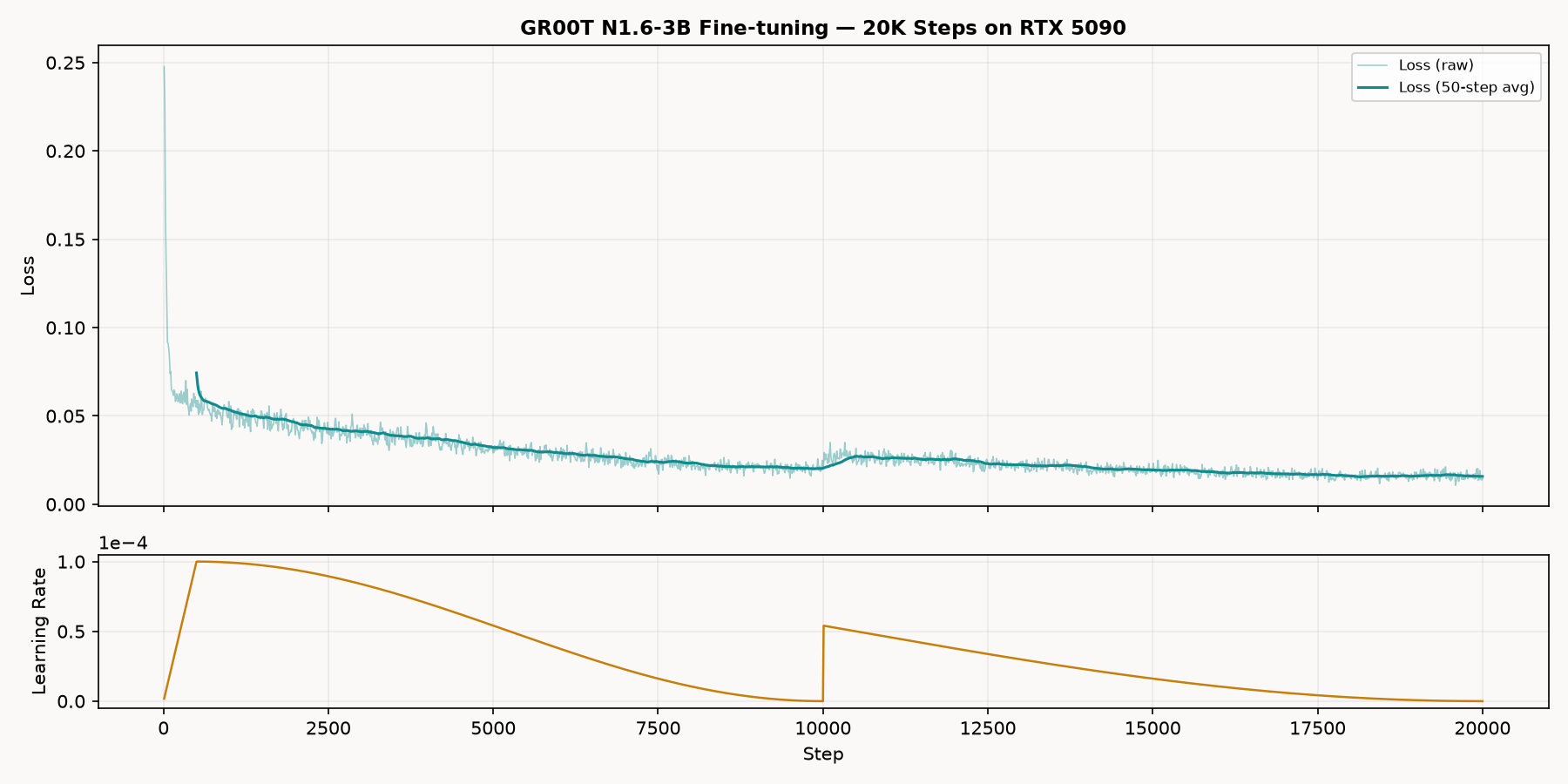
Training loss and learning rate over 20K steps. The upper panel shows raw loss (light) and 50-step moving average (solid). Loss drops from 0.25 to 0.05 in the first 1K steps as the diffusion head learns the action distribution, then gradually settles to 0.02 by step 10K. At step 10K, training resumes from a checkpoint with a fresh cosine schedule at half the peak LR (5e-5), pushing loss down to 0.015. The lower panel shows the cosine learning rate decay with 5% warmup, and the visible discontinuity at the checkpoint resume.
Train loss: 0.010 (average). Training throughput: 150 samples/sec, 2.3 steps/sec. Total wall time: 2.4 hours.
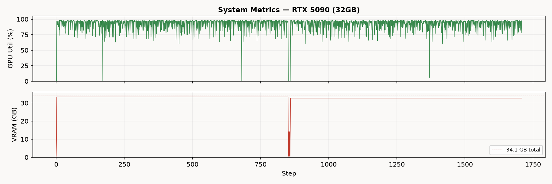
RTX 5090 system metrics during training. GPU utilization (top) holds above 90% for nearly the entire run, with brief dips during checkpoint saves every 2K steps. The VRAM plot (bottom) shows the card running at 33.5 GB out of 34.1 GB available. The drop to zero around step 850 corresponds to the checkpoint resume, where PyTorch deallocates and reallocates the full model. I needed expandable_segments:True to survive this reallocation without OOM.
Real robot evaluation
I evaluate with FRAME robotics metrics, logged to MLflow. Each rollout records per-joint trajectories (commanded vs observed), computes FRAME metrics (path length, smoothness, DTW, ATE, RTE, action MSE), and generates tracking error plots. All figures and scalar metrics are logged as MLflow artifacts for comparison across runs.
I ran 5 eval rollouts across different checkpoints and configurations. The table below shows the key metrics:
| Run | Checkpoint | Success | Action MSE | Gripper MSE | Path Smoothness |
|---|---|---|---|---|---|
| Recording demo | finetune_cotrain/ckpt-20000 | 1/1 | 87.3 | 75.9 | 0.73 |
| Jul 4 eval | finetune_cotrain/ckpt-20000 | 1/1 | 84.6 | 69.5 | 0.72 |
| Active-gripper fail | finetune_cotrain/ckpt-20000 | 0/1 | 124.0 | 109.8 | 0.72 |
| Trajectory fail | finetune_cotrain/ckpt-20000 | 0/1 | 102.5 | 87.7 | 0.74 |
| Inactive-gripper fail | so101_finetuned/ckpt-20000 | 0/1 | 6.7 | 0.2 | 0.45 |
The two successful runs and three failure modes tell different stories. Here is the full MLOps breakdown.
Successful run (video recording session)
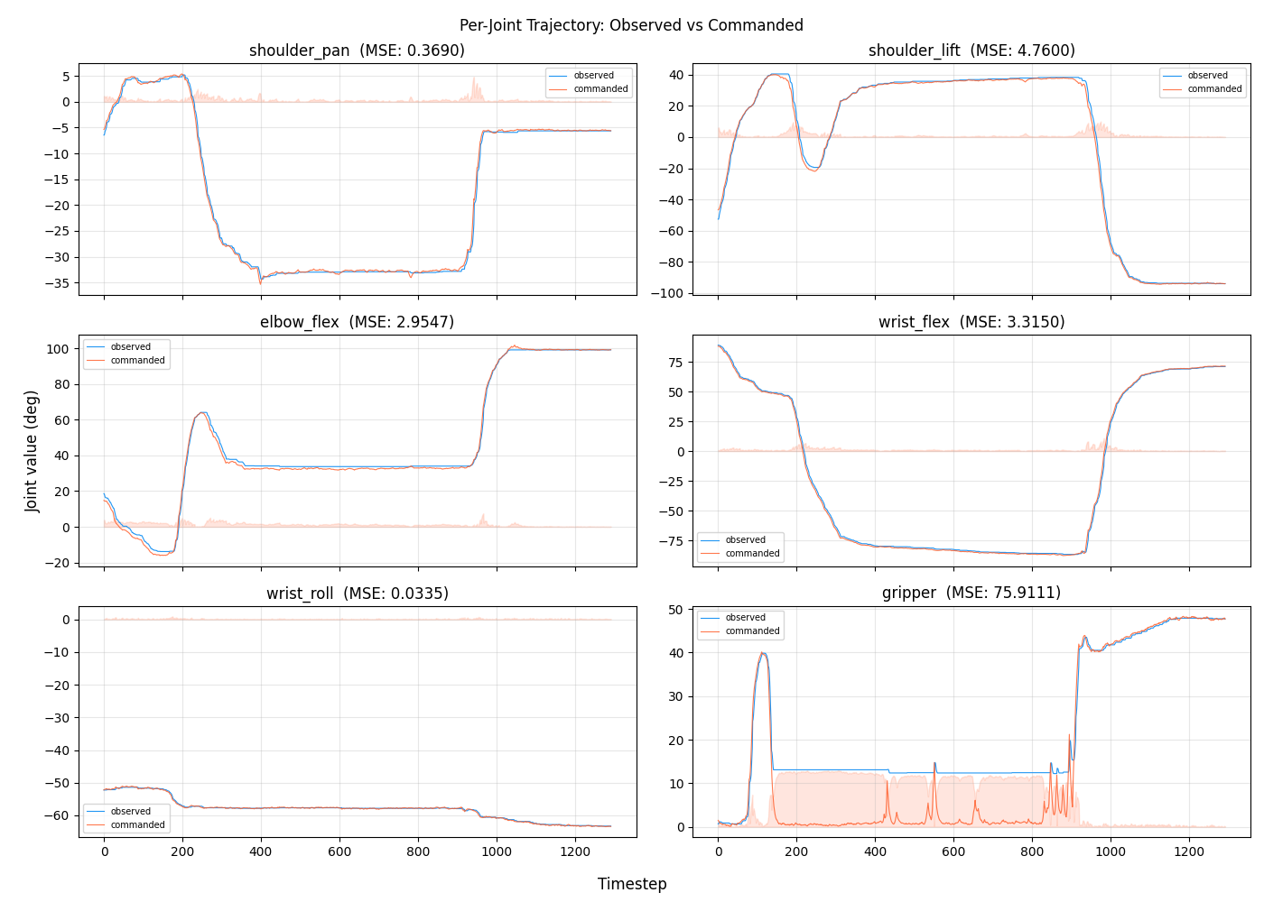
Per-joint trajectory: commanded (orange) vs observed (blue). Each subplot shows one of the 6 joints over 1293 timesteps. The arm joints (shoulder_pan through wrist_roll) show tight tracking with MSE under 5. The gripper panel (bottom right, MSE=75.9) shows two clear open/close cycles: the first spike around step 150 is the grasp open, the second around step 900 is the release open for placing. Between cycles, the gripper holds at 10-15 degrees (closed on the vial). The commanded signal lags slightly behind observed because of the EMA smoothing (alpha=0.2) applied between action chunks.
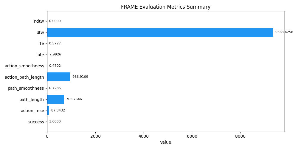
FRAME metrics summary. DTW (9363) measures cumulative trajectory alignment between commanded and observed paths. Path length (704) vs action path length (967) shows the policy commands more motion than the robot executes, since EMA smoothing absorbs small corrections. RTE (0.57) is low, meaning endpoint error stays small. Success = 1.0.
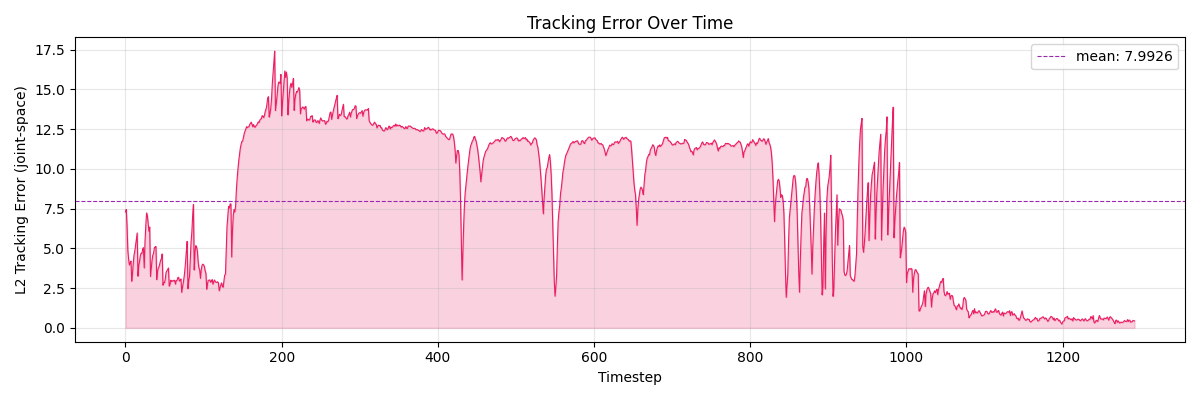
L2 tracking error over time. Error is low (2-5) during approach, spikes to 12-15 during the grasp and place phases when the gripper is actively opening/closing (contributing most of the MSE), and drops back to near zero after the vial is placed. Mean ATE = 7.99.
Earlier successful eval (Jul 4)
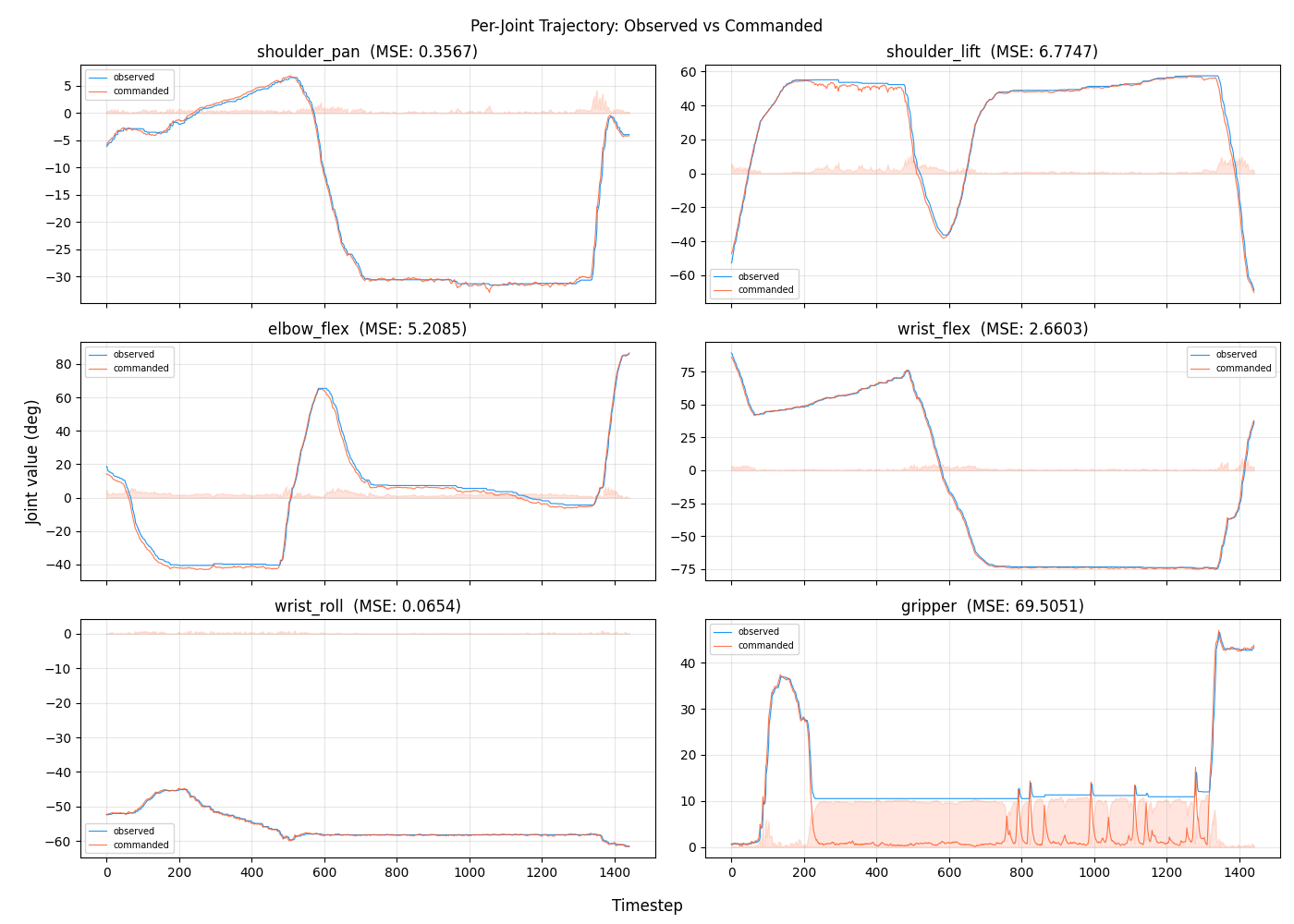
Per-joint trajectory from the first successful evaluation. Same checkpoint, similar pattern. The shoulder_pan range is narrower (5 to -30 degrees) compared to the recording run (5 to -35 degrees), reflecting a slightly different vial starting position. Gripper MSE is 69.5 with the same two-cycle open/close pattern. The wrist_roll channel is nearly flat (MSE=0.07), confirming that the 5th DOF barely contributes to this task.
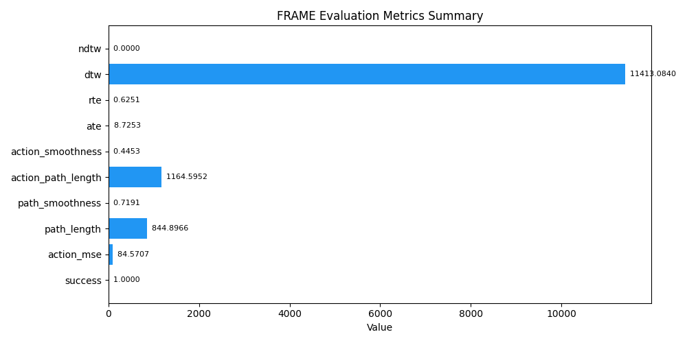
FRAME metrics. DTW is higher (11413 vs 9363) because this rollout ran longer (1450 steps vs 1293). Path smoothness (0.72) is consistent across both successful runs, suggesting the EMA setting produces stable motion regardless of episode length.
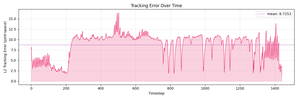
Tracking error. Mean ATE = 8.73. The error profile is noisier than the recording run, with sustained 10-12 error between steps 400-1200. The gripper's constant open/close adjustments during the hold phase contribute to this baseline error.
Failure mode 1: active gripper, bad trajectory
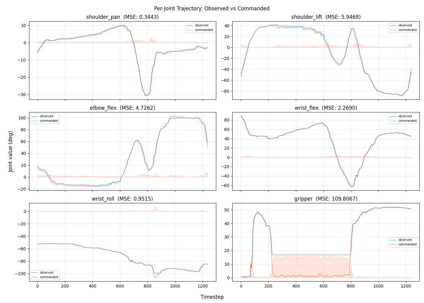
Active gripper but failed task. The gripper channel (MSE=109.8) shows strong open/close commands, even more aggressive than the successful runs. But look at the elbow_flex and wrist_flex panels: the arm moves through its full range and ends at the joint limits (elbow at 100 degrees, wrist at 75 degrees). The policy commanded a valid pick but the place trajectory drove the arm into a kinematic singularity near the workspace boundary. This is a trajectory planning failure, not a gripper failure.
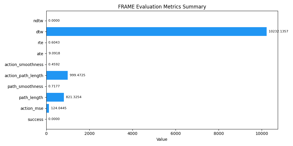
FRAME metrics. Action MSE (124.0) is the highest across all runs. The high action_path_length (999) vs path_length (821) shows the policy is commanding large corrections that the robot cannot fully execute, a sign that the arm is fighting joint limits.
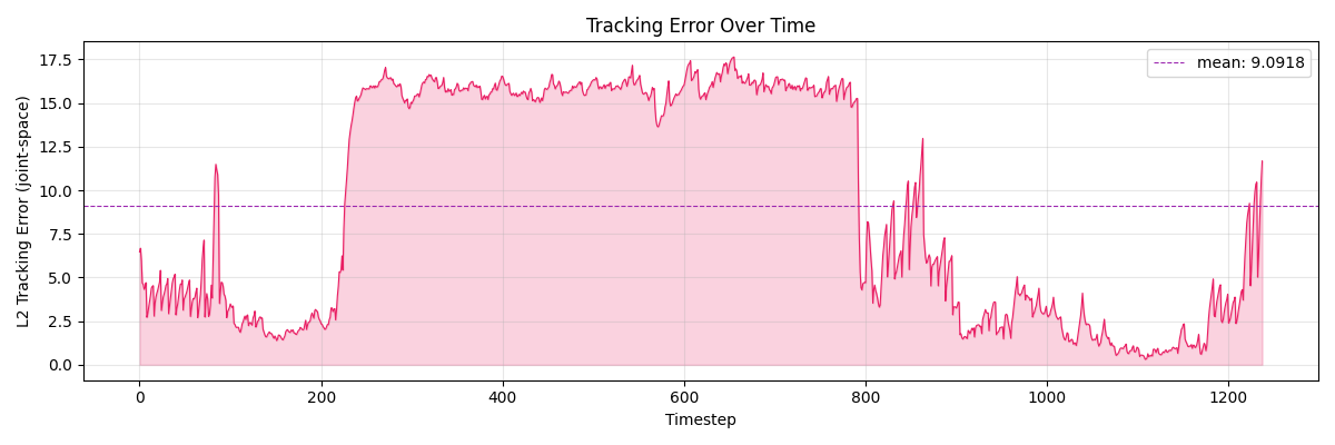
Tracking error. Error plateaus at 15-17 between steps 250-800 (during the place attempt), far above the 10-12 plateau in successful runs. This sustained high error is the arm stuck near joint limits, unable to track the commanded trajectory.
Failure mode 2: inactive gripper (different checkpoint)
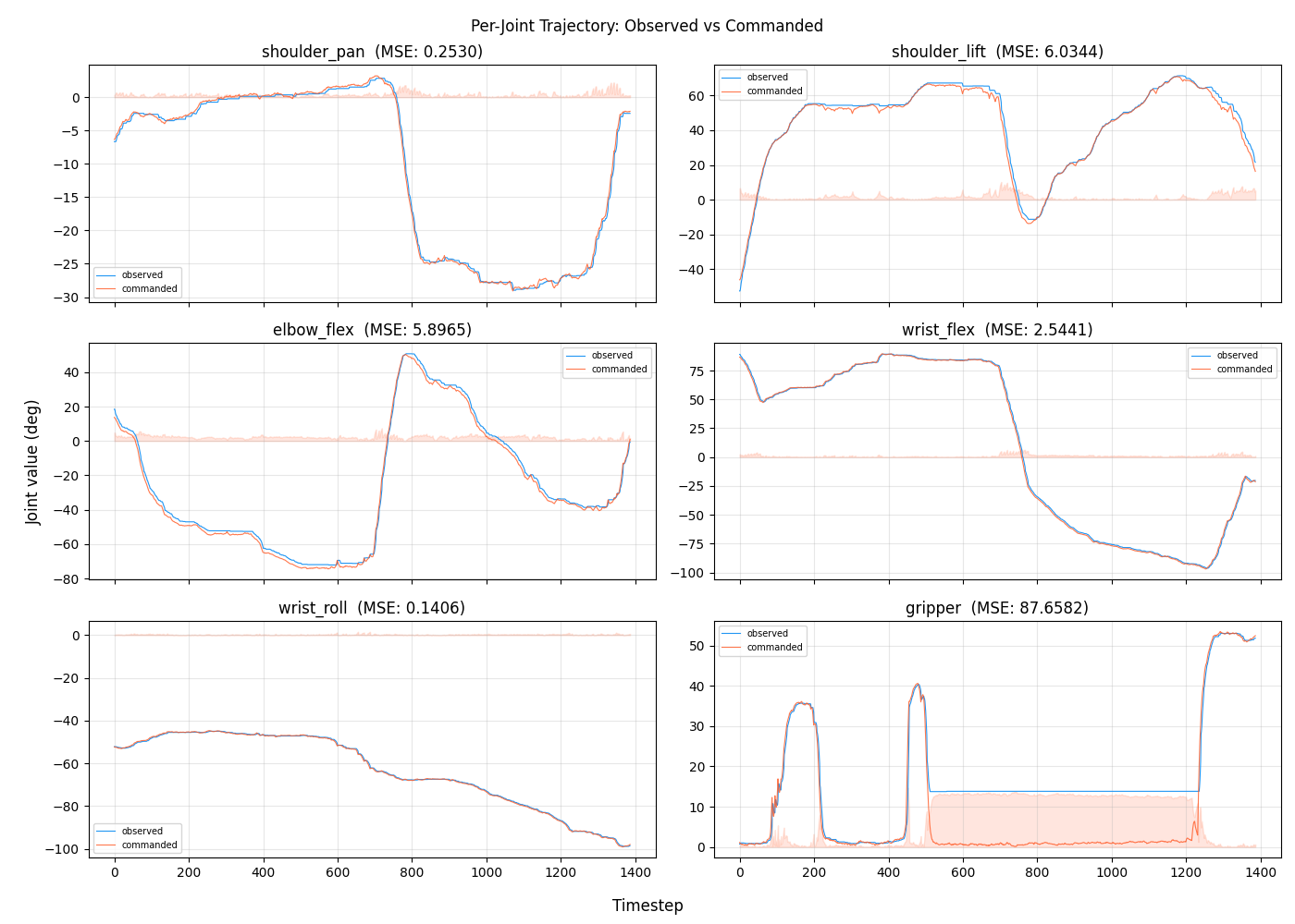
The gripper channel tells the whole story. This is a different checkpoint (`so101_finetuned`, trained without real co-training data). The arm joints show reasonable motion with similar shapes to successful runs. But the gripper (MSE=87.7) opens for the grasp and then enters a sustained hold at 10-15 degrees from step 400 onward, without the second open/close cycle needed for placing. The policy learned to pick but not to release.
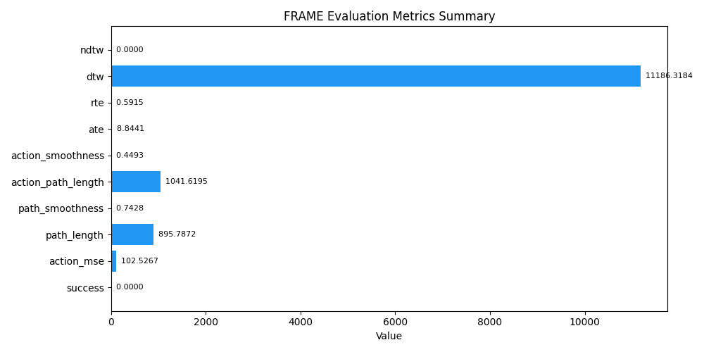
FRAME metrics. Action MSE (102.5) is between the successful runs and the joint-limit failure. Path smoothness (0.74) is actually the highest across all runs because the arm motion is smooth; it just does not complete the task. Smoothness alone is not a success indicator.
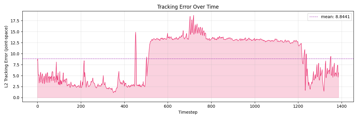
Tracking error. The error spikes to 15-18 during the place phase (steps 600-800) and stays elevated because the arm is trying to place while the gripper has not released. Mean ATE (8.84) is close to successful runs, which is why aggregate metrics alone miss the failure.
Deploying to the real robot
Inference runs as a ZMQ server in a separate container. The policy container loads the fine-tuned checkpoint and listens on port 5555. The robot container connects as a client and runs the control loop at 30 Hz:
- Read 6 joint positions + 3 camera frames
- Package into GR00T format:
{video, state{arm(5), gripper(1)}, language} - Send to policy server, receive action chunk of 8 timesteps
- Apply EMA smoothing (alpha=0.2) between consecutive chunks
- Send motor commands to Feetech servos
The action horizon drops from 16 (simulation) to 8 (real) for safety. Fewer predicted steps means more frequent policy queries and faster correction of tracking errors. The EMA smoothing prevents jitter at chunk boundaries where consecutive predictions might disagree.
The entire deployment is containerized: ./real launches the robot container with device access, ./policy launches the inference server with GPU access. Both share the model directory via bind mount. No pip installs at runtime, no environment conflicts.
What I learned
Config-driven everything. Every parameter (joint limits, camera poses, physics masses, DR ranges, training hyperparams, eval defaults) lives in one of 11 YAML files. When I needed to change rack mass from 2.0kg to 0.2kg, it was a one-line YAML edit, not a code change. When I needed to swap IK backends, same thing. The upfront cost of building the config system paid back immediately.
Gripper MSE as a diagnostic. During eval, I discovered that per-joint MSE decomposition is the most useful diagnostic for policy debugging. A model that “moves but doesn’t grasp” shows near-zero gripper MSE because the gripper is not being commanded at all. A working model has high gripper MSE because it is actively opening and closing. I saw this directly: a degraded checkpoint had gripper MSE of 0.2 (failed every trial); the working checkpoint had 69.5 (succeeded).
Contact physics matters more than rendering fidelity. I spent time on photorealistic rendering, domain randomization, and color jitter. The bug that actually blocked real-robot success was a 2cm PhysX contact offset making the gripper push objects away at distance. The sim-to-real gap is not always visual.
5 DOF is enough. The SO-101 cannot independently control all 6 DOF of end-effector pose. But with proper task-space weighting and adaptive rotation scaling, 5 DOF handles pick-and-place reliably. The constraint forced us to build better IK controllers that would generalize to any kinematically limited system.
The full pipeline, from 130 sim seeds + 20 real demos to a working policy on the real robot, takes about 4 hours: 30 minutes of data generation, 1 hour of rendering, 2.4 hours of training, and 30 minutes of eval. The workshop is designed so someone can run this end-to-end in a single session on a single GPU.
Enjoy Reading This Article?
Here are some more articles you might like to read next: